ClonEvol
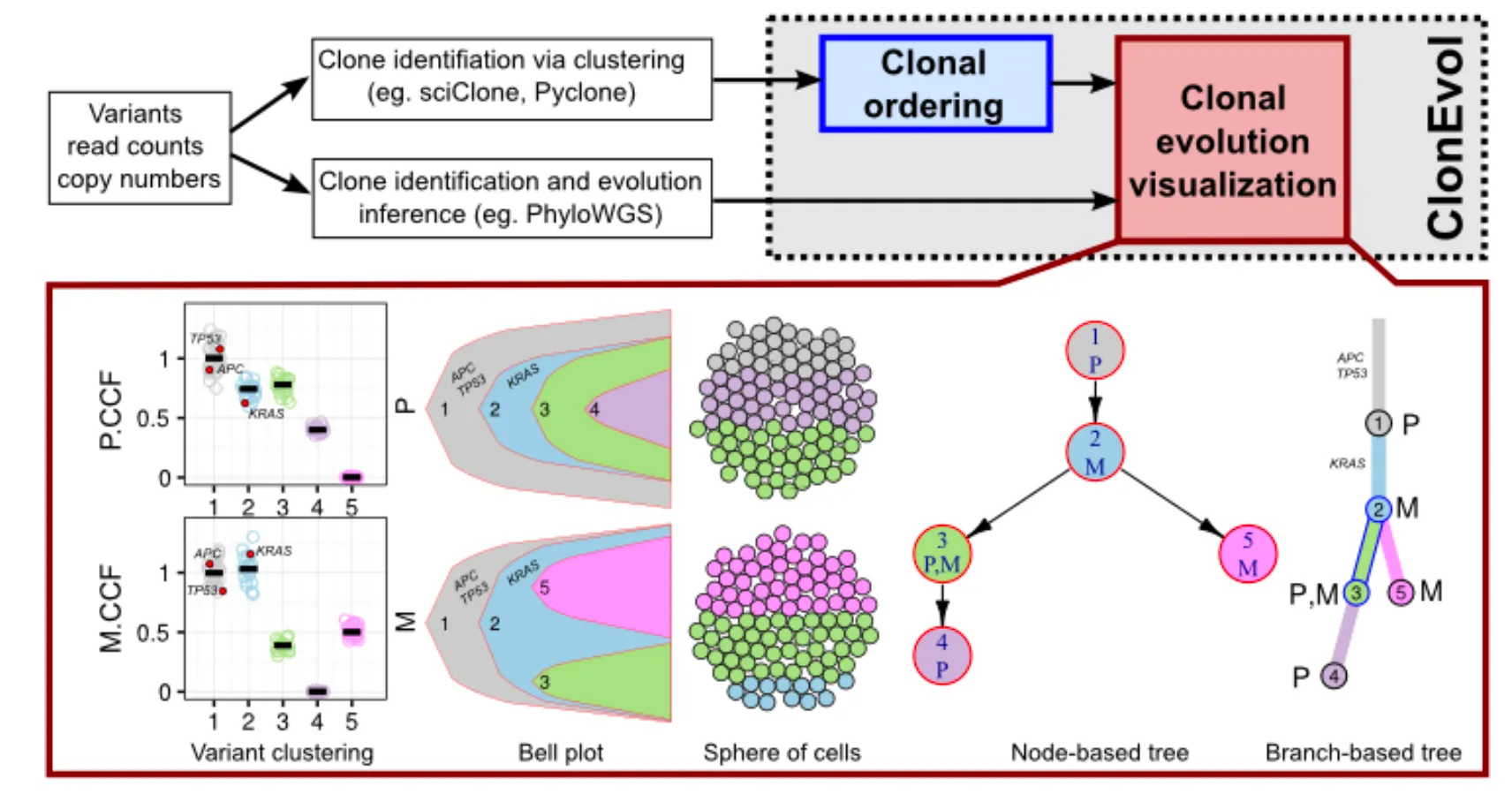
ClonEvol is a package for clonal ordering and clonal evolution visualization. It uses the clustering of heterozygous variants identified using other tools as input to infer consensus clonal evolution trees and estimate the cancer cell fraction.
Installation
install.packages('devtools')
library(devtools)
install_github('hdng/clonevol')
install.packages('gridBase')
install.packages('gridExtra')
install.packages('ggplot2')
install.packages('igraph')
install.packages('packcircles')
install_github('hdng/trees')
R
복사
Manual
Input data
ClonEvol requires an input data frame consisting of at least a cluster column and one or more variant cellular prevalence columns, each corresponds to a sample. The cluster should be named by contiguous integer numbers, starting from 1. For better visualization, the names of the cellular prevalence columns should be short.
# Shorten vaf column names as they will be.
vaf.col.names = grep('.vaf', colnames(x), value=T)
sample.names = gsub('.vaf', '', vaf.col.names)
x[, sample.names] = x[, vaf.col.names]
vaf.col.names = sample.names
# Prepare sample grouping.
sample.groups = c('P', 'R')
names(sample.groups) = vaf.col.names
# Setup the order of clusters to display in various plots (later)
x = x[order(x$cluster), ]
R
복사
필요한 column들 (PyClone의 경우 loci별로 build_table 해야 한다.)
•
cluster index를 나타내는 column
•
VAF 값들을 나타내는 column들
Input data 만들 때 매우 중요함!!!
Cluster ID를 부여할 때, subclone size가 작아지는 순서대로 1, 2, 3, ... 으로 부여해야 tree가 제대로 그려진다.
Visualizing the variant clusters
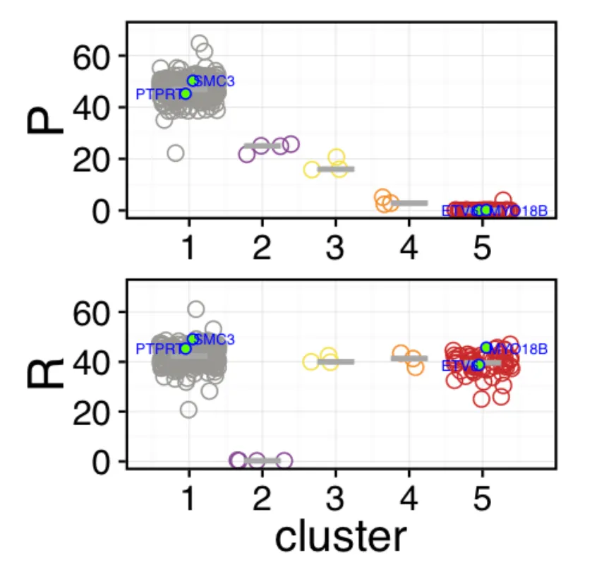
The following code will plot the clustering results for you to investigate. It will plot the cellular prevalence of the variants across clusters and samples, using jitter, box and violin plots to allow close investigation of the clustering. This plot is very powerful as it can visualize lots of samples and clusters at once.
pdf('box.pdf', width = 3, height = 3, useDingbats = FALSE, title='')
pp <- plot.variant.clusters(x,
cluster.col.name = 'cluster', # Cluster index를 나타내는 colname.
show.cluster.size = FALSE,
cluster.size.text.color = 'blue',
vaf.col.names = vaf.col.names, # VAF를 나타내는 colname들. 여기서는 P,R
vaf.limits = 70,
sample.title.size = 20,
violin = FALSE,
box = FALSE,
jitter = TRUE,
jitter.shape = 1,
jitter.color = clone.colors,
jitter.size = 3,
jitter.alpha = 1,
jitter.center.method = 'median',
jitter.center.size = 1,
jitter.center.color = 'darkgray',
jitter.center.display.value = 'none',
highlight = 'is.driver', # Boolean column으로 highlight.
highlight.shape = 21,
highlight.color = 'blue',
highlight.fill.color = 'green',
highlight.note.col.name = 'gene', # Highlight되는 row표시를 어떤 col로 할지.
highlight.note.size = 2,
order.by.total.vaf = FALSE)
dev.off()
R
복사
Clonal ordering with ClonEvol
Inferring clonal evolution trees
At this step, we assume that you already thorougly looked at your clustering and feel confident about it. Let's tell ClonEvol to perform clonal ordering and construct the consensus trees. In this example AML1 case, we will use VAF of variants. If your data contain copy-altered variants and copy number corrected CCF estimated by the clustering tool (e.g., PyClone), you can provide the corrected CCF to ClonEvol via ccf.col.names parameter in infer.clonal.models function, or calculate the equivalent copy number corrected VAF as half of the CCF.
y = infer.clonal.models(
variants = x,
cluster.col.name = 'cluster',
vaf.col.names = vaf.col.names,
sample.groups = sample.groups,
cancer.initiation.model='monoclonal',
subclonal.test = 'bootstrap',
subclonal.test.model = 'non-parametric',
num.boots = 1000,
founding.cluster = 1,
cluster.center = 'mean',
ignore.clusters = NULL,
clone.colors = clone.colors,
min.cluster.vaf = 0.01,
# min probability that CCF(clone) is non-negative
sum.p = 0.05,
# alpha level in confidence interval estimate for CCF(clone)
alpha = 0.05
)
R
복사
The infer.clonal.models function takes the clustering results and evaluates all clonal orderings to reconstruct the clonal evolution trees and estimate the CCF of the clones in individual samples. Several important parameters are:
•
variants: the variant clustering data frame
•
cluster.col.name: name of the cluster column
•
vaf.col.names: names of VAF columns
•
sum.p: min probability that a CCF estimate for a clone in a sample is non-negative in an accepted clonal ordering
•
alpha: alpha level, or [1 - confidence level] for CCF estimate of a clone.
Mapping driver events onto the trees
If the previous step succeeds and gives you a tree or several trees (congrats!), we can next map some driver events onto the tree to make sure they wil be visualized later. For AML1 case, column is.driver indicates if the variant is a (potential) driver event. We will use the gene name in column gene to annotate the variants in the tree.
y = transfer.events.to.consensus.trees(
y,
x[x$is.driver, ],
cluster.col.name='cluster',
event.col.name='gene',
)
R
복사
Converting node-based trees to branch-based trees
ClonEvol can plot both node-based tree (each clone is a node), or branch-based tree (each branch represents the evolution of a clone from its parental clone, and each node represents a point where the clone is established/founded). Before we can draw the latter tree, we need to preprare it.
y = convert.consensus.tree.clone.to.branch(
y,
branch.scale='sqrt',
)
R
복사
plot.clonal.models(
y,
# box plot parameters
box.plot = TRUE,
fancy.boxplot = TRUE,
fancy.variant.boxplot.highlight ='is.driver',
fancy.variant.boxplot.highlight.shape = 21,
fancy.variant.boxplot.highlight.fill.color ='red',
fancy.variant.boxplot.highlight.color ='black',
fancy.variant.boxplot.highlight.note.col.name ='gene',
fancy.variant.boxplot.highlight.note.color ='blue',
fancy.variant.boxplot.highlight.note.size = 2,
fancy.variant.boxplot.jitter.alpha = 1,
fancy.variant.boxplot.jitter.center.color ='grey50',
fancy.variant.boxplot.base_size = 12,
fancy.variant.boxplot.plot.margin = 1,
fancy.variant.boxplot.vaf.suffix ='.VAF',
# bell plot parameters
clone.shape ='bell',
bell.event = TRUE,
bell.event.label.color ='blue',
bell.event.label.angle = 60,
clone.time.step.scale = 1,
bell.curve.step = 2,
# node-based consensus tree parameters
merged.tree.plot = TRUE,
tree.node.label.split.character = NULL,
tree.node.shape ='circle',
tree.node.size = 30,
tree.node.text.size = 0.5,
merged.tree.node.size.scale = 1.25,
merged.tree.node.text.size.scale = 2.5,
merged.tree.cell.frac.ci = FALSE,
# branch-based consensus tree parameters
merged.tree.clone.as.branch = TRUE,
mtcab.event.sep.char =',',
mtcab.branch.text.size = 1,
mtcab.branch.width = 0.75,
mtcab.node.size = 3,
mtcab.node.label.size = 1,
mtcab.node.text.size = 1.5,
# cellular population parameters
cell.plot = TRUE,
num.cells = 100,
cell.border.size = 0.25,
cell.border.color ='black',
clone.grouping ='horizontal',
#meta-parameters
scale.monoclonal.cell.frac = TRUE,
show.score = FALSE,
cell.frac.ci = TRUE,
disable.cell.frac = FALSE,
# output figure parameters
out.dir ='output',
out.format ='pdf',
overwrite.output = TRUE,
width = 8,
height = 4,
# vector of width scales for each panel from left to right
panel.widths =c(3,4,2,4,2)
)
R
복사

