Table of contents
Highly accurate protein structure prediction with AlphaFold
Article
Supplementary material
Summary
아미노산 residue들의 co-evolution, residue pair의 feature 및 두 요소 간의 상호작용을 deep learning 모델에 접목시켜 protein structure를 예측하기 위해서 self-attention과 그 variant들을 훌륭하게 design하여 활용함
Introduction
Seven novelties suggested by authors
저자들은 AlphaFold2 모델의 novelty로서 7가지를 제시한다.
1.
Multiple sequence alignments (MSAs)와 pairwise feature를 jointly embed할 수 있는 new architecture
2.
New output representation과 associated loss
→ Backbone frame (for residue) and torsion angle (for atom)
→ End-to-end structure prediction을 가능하게 함.
3.
New equivariant attention architecture
→ 두 residue의 3차원 공간 상의 거리를 attention에 반영할 수 있다. 이 때, whole protein이 공간 상에 어떻게 위치하는지(global transformation)는 attention에 영향을 주지 않는다.
→ (global transformation-) invariant point attention (IPA)
4.
Intermediate loss의 사용
→ prediction들의 iterative refinement를 가능하게 함.
5.
Masked MSA loss
→ BERT를 떠올리면 된다. 고의로 MSA의 residue 일부를 masking해놓고 이를 reconstruct하도록 만드는 loss. BERT-loss
6.
Learning from unlabelled protein sequences using self-distillation
→ Noisy student self-distillation
참고 논문: Self-training with Noisy Student improves ImageNet classification (CVPR 2020)
7.
Self-estimates of accuracy
→ 예측된 구조의 residue 별로 AlphaFold2의 예측을 얼마나 신뢰할 수 있는지 스스로 판단하는 방법을 제시함.
→ per-residue accuracy of the structure (pLDDT)
AlphaFold2와 기존 AlphaFold, 그리고 다른 방법들과의 차이점은?
1.
Feature representation 수준의 차이
가장 먼저 AlphaFold의 feature representation 방법을 간단히 살펴보자. AlphaFold의 input은 의 3차원 matrix이며, 이 때 은 input amino acid sequence의 길이, 는 feature 종류의 개수이다.
주목할 점은 feature는 그 특성에 따라서 각 residue 마다 부여되는 feature (sequence-length features라고 부르며, MSA feature를 포함한다)와 residue pair에 부여되는 feature (sequence-length-squared features, covariation features, or pair features)로 나뉠 수 있다. Pair feature를 형태로 나타내는 것은 straightforward하다. 하지만 sequence-length features를 로 나타내는 방법은 생각해내기 나름이다. AlphaFold의 경우는 간단하게 feature들을 tiling하여 로 만들었다 (그림 참조)
AlphaFold 2의 경우는, 다음 section의 개요도에서도 알 수 있듯이, MSA feature와 pair feature를 각각 embedding하고, 심지어 Evoformer 구조를 통하여 두 feature간의 information exchange가 일어날 수 있도록 하여 개별적이지만, joint하게 embedding을 수행한다.
분야 history에 대한 research를 많이 해보지 않아서 100% 확신할 수는 없지만, deep learning + protein structure prediction 관련 기존 논문들에서 AlphaFold2와 같이 MSA / pair-representation을 독립적으로 embedding하되 상호 보완적인 information exchange가 일어날 수 있도록 모델을 구성한 경우는 없다.
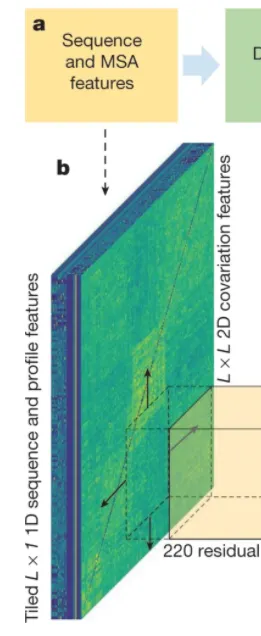
AlphaFold input features. L x 1 feature를 tiling하여 L x L 형태로 만들었음에 주목하자.
2.
AlphaFold2는 end-to-end model 이다.
AlphaFold , trRosseta (Yang et al., PNAS, 2019) 등의 deep learning 기반 protein structure prediction 기법들은 end-to-end 라고 보기 어렵다. 이들은 먼저 MSA, residue pair feature 등을 이용하여 residue 사이의 distance(혹은 all-pair distance를 나타내는 distogram)를 예측하는 deep learning 모델을 학습시키고, 해당 모델로부터 예측된 distogram을 만족하는 다양한 protein structure 중 최소의 potential energy를 가지는 structure를 찾는 문제를 optimization 문제로 formulation하여 풂으로써 final protein structure를 얻는다. 즉, end-to-end가 아닌 distogram prediction → protein structure optimization 의 two-step procedure라고 봐도 무방할 듯 하다.
한편, AlphaFold2의 protein structure prediction은 먼저 residue 각각의 위치를 (의 backbone frame tuple (이것은 Euclidean transformation, rigid transformation의 형태다) 로 나타내고, residue가 rigid하다는 가정 하에, residue 의 location과 orientation이 결정되면 residue 내 각 원자의 위치는 오로지 torsion angle에 의해서 결정된다는 사실을 이용한다. 따라서 backbone frame을 어떻게 rotation할 것이며 어느 방향으로 얼만큼 translation할지 결정하는 transform을 학습하고, 나아가 각 residue atom의 torsion angle을 학습하면 마침내 3차원 공간 내에서의 개별 atom의 위치를 얻는다. 이 위치를 정답과 비교하여 loss를 계산하고 (loss에 관해서는 아래에서 자세히 살펴보자), backprop 시키면 결과적으로 end-to-end model로서 학습이 가능해진다.
AlphaFold2 structure
Supplementary material에 모델 구현이 아주 상세하게 설명되어 있다. 구조가 복잡하기 때문에 큰 단위의 모델 설계부터 상세한 구조 및 연산까지 top-down 방식으로 차근차근 알아보자.
Model I/O and overview of the structure
이 section에서는 AlphaFold2 모델이 크게 어떠한 부분들로 구성되며, 각 부분의 input/output 형식이 어떻게 되는지 알아보고, 더불어 간단하게 그 의미를 파악해 본다.
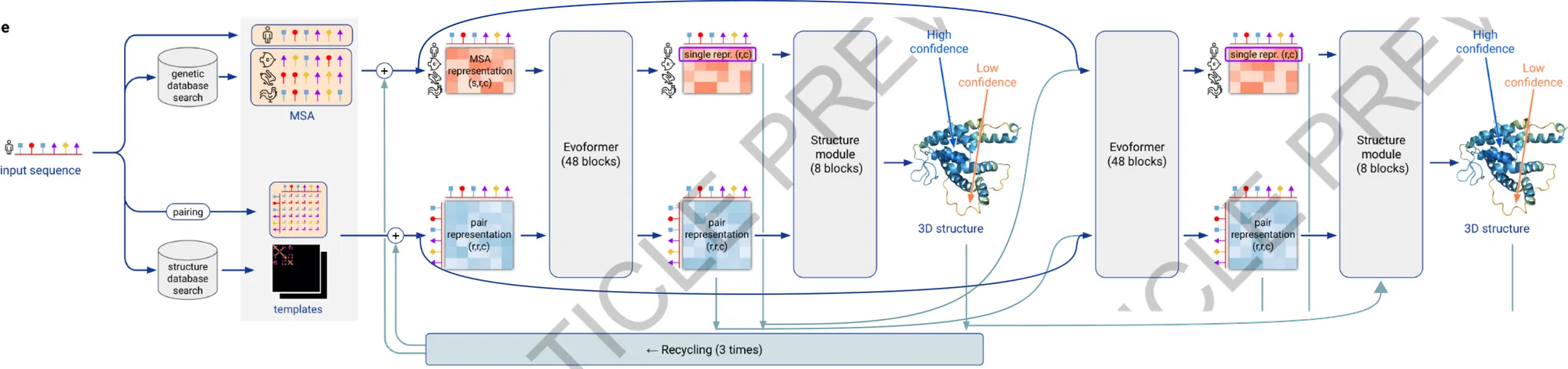
AlphaFold2 모델은 크게 아래와 같이 나타낼 수 있다.
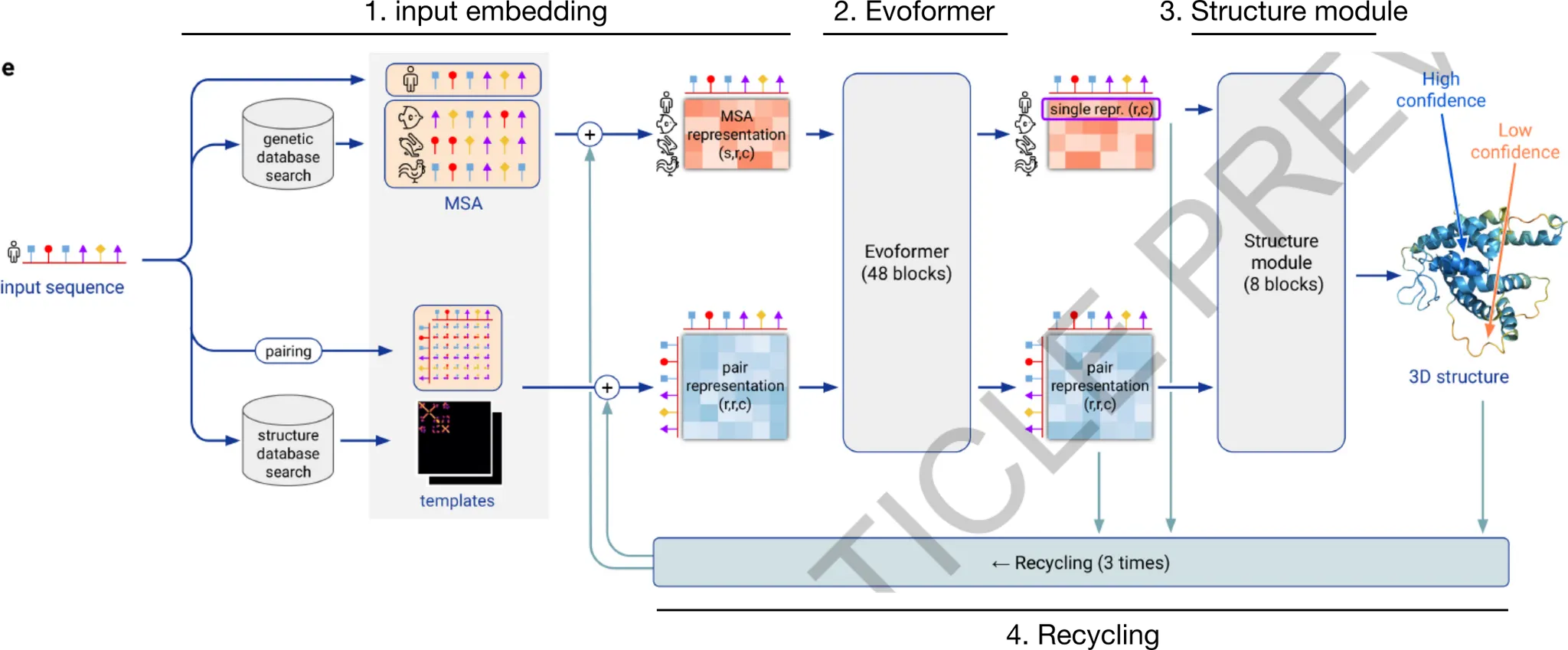
AlphaFold2 model의 개요. 모델은 크게 4가지 부분으로 구성된다. (1) input embedding, (2) Evoformer, (3) Structure Module, (4) Recycling.
이를 직관적으로 해석하자면 다음과 같다. 크게 보면 (1) input sequence와 evolutionary relationship을 보이는 다른 종의 sequence 정보(MSA의 형태로)를 이용하고, input sequence의 구조 예측에 도움을 줄 수 있는, 이미 알려진 protein structure template를 이용하여 input sequence가 나타내는 3D structure를 예측하고자 한다. 그 과정에서 (2) Evoformer는 MSA embedding과 residue pair embedding의 self-attention update와 더불어, 서로 간의 information exchange를 거듭하며(x48회) embedding을 update하고, (3) Structure module에서는 Evoformer의 결과로 나타난 embedding들을 이용하여 structure를 예측한다. (4) 한편, 추가적인 성능 향상을 위해서 MSA와 pair representation, 그리고 예측된 protein structure를 다시 활용하여 새로운 예측을 하는 방법으로 prediction의 refinement를 도모한다 (recycling).
AlphaFold2 모델 전체의 input/output은 간단하다. Input으로는 query amino acid sequence가 들어오고, output으로는 각 heavy atom(=H가 아닌 atom)의 position과, per-residue accuracy of the structure(pLDDT)를 출력한다.
Shortcut
Input embedding의 개요

Input - amino acid sequence
Output - MSA representation ( & residue pair representation (
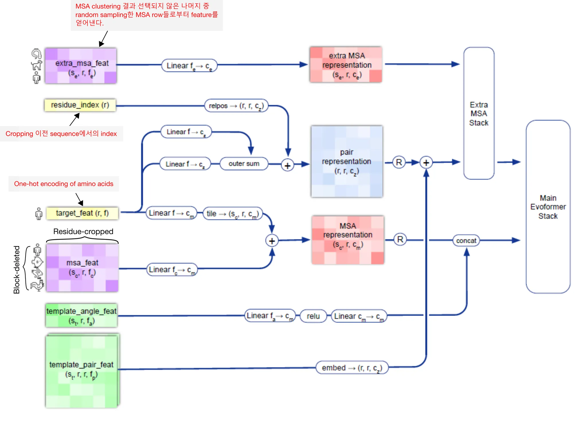
Main Evoformer stack으로 들어갈 input feature들을 준비하는 부분이다. Input amino acid sequence로부터 MSA representation (과 residue pair representation ( matrix들을 만들어내게 된다.
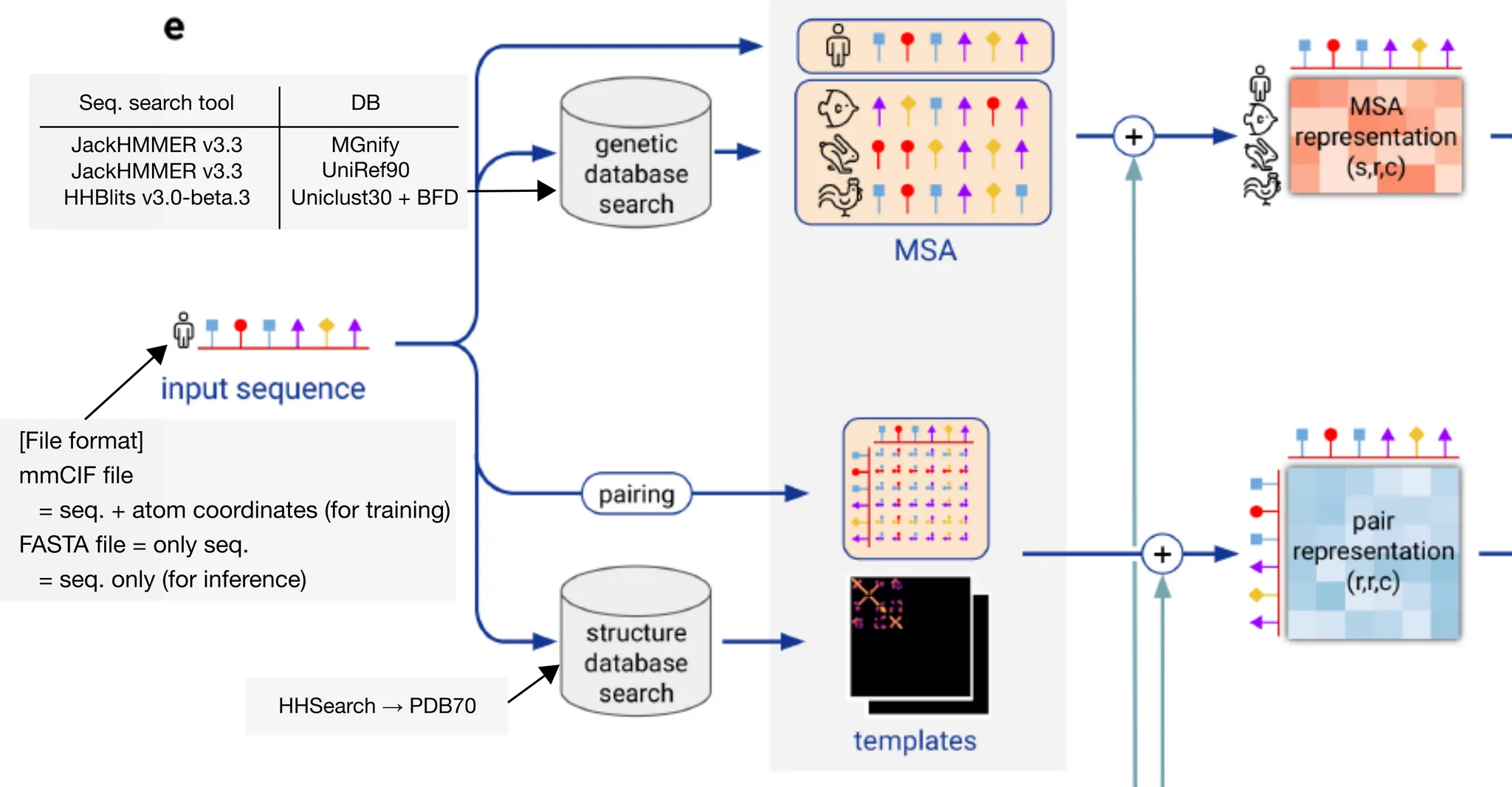
Input embedding의 개요. Input amino acid sequence를 받아서 어떻게 MSA feature와 residue pair feature를 만들어내는지에 주목하자.
Input amino acid sequence가 들어오면, 가장 먼저 JackHMMER와 HHBlits를 이용하여 sequence DB에 검색을 수행한다. 그 결과물로 sequence들의 multiple sequence alignment(MSA)를 얻는다 (Genetic search). 다음으로, UniRef90 search 결과로 얻은 MSA를 이용하여 PDB70 데이터베이스를 HHSearch 를 이용하여 검색, residue 일부와 matching되어 structure에 대한 힌트를 제공하는 template를 얻는다. (Template search). 이후 일련의 preprocessing 과정을 거쳐 MSA representation과, residue pair representation을 얻는다.
Evoformer stack의 개요
Input - MSA representation ( & residue pair representation ( (+ Recycled input)
Output - (Updated) MSA representation & (Updated) pair representation
MSA representation과 pair representation의 information exchange/communication 을 통하여 evolutionary relationship과 spatial relationship을 상호보완적으로 반영시켜 MSA/pair representation을 update한다.
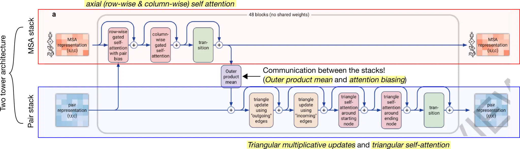
Evoformer stack의 개요. Evoformer stack은 크게 볼 때 two-tower architecture를 취한다. Tower 하나는 MSA embedding을 update하는 MSA stack이고, 다른 하나는 amino acid pair representation를 update하는 pair stack이다. 눈여겨볼 점은 두 stack 사이의 information exchange가 일어날 수 있도록, outer product mean과 attention biasing을 골자로 하는 연산이 중간에 들어간다는 것이다. 각 stack의 주요 연산을 노란색 highlight 해 두었다. MSA stack의 경우 axial gated self-attention, 즉 row-wise (sequence-wise) gated attention → column-wise (residue-wise) gated attention을 주요 연산으로 한다. Pair stack의 경우 triangular multiplicative updates 와 triangular self-attention 을 주요 연산으로 한다. 자세한 것은 아래에서 살펴보도록 하자.
참고) Axial attention 연산에 대한 설명
Pseudocode - Evoformer stack
Structure Module의 개요
Input - Evoformer로 update된 single (query) MSA representation () & pair representation ( (+ Recycled input)
Output - 3D atom coordinate, residue 단위의 confidence (pLDDT), Losses
Structure module은 아래와 같이 간단히 나타낼 수 있다. 이 module은 직접적으로 protein의 3차원 구조, 즉 protein을 이루는 heavy atom들의 3D coordinate을 예측한다. 이 예측은 residue position 예측 → atom position 예측의 two-step procedure라고 생각하면 쉬운데, 보다 구체적으로 알아보자.
Residue의 orientation과 position은 (회전변환, 평행이동) 을 나타내는 ( 형태의 Euclidean transformation 으로 나타낼 수 있다. 처음에는 모든 atom이 identity transform으로 initialize 되며 (모든 residue가 한 점에 모여 있어서 'black-hole initialization'이라고 부른다), 이후 iteration을 돌면서 residue의 위치와 orientation을 update하는 'Update transformation'을 MSA single representation으로부터 예측, 이를 기존 transformation에 반복적으로 적용해나가면서 residue 수준의 structure를 update하는 것이다. Residue 수준의 structure가 결정되면, atom 수준의 position은 torsion angle에 의해서만 결정된다고 본다. (Rigid-body assumption에 의해서) 따라서 MSA single representation으로부터 atom의 torsion angle들 또한 예측하여 atom의 position이 예측될 수 있는 것이다.
이 과정에서, MSA single representation은 invariant point attention module에 의해서 지속적인 self-attention update를 거치게 된다. 이 self-attention의 bias로서 pair representation이 사용되며, 현재까지 예측된 residue backbone frame의 위치 정보 또한 활용되어 3D space 내에서의 amino acid proximity 자체가 attention에 직접적으로 반영될 수 있게 한다.
Torsion angle / Dihedral angle에 대한 설명
Shotcuts
Recycling
Evoformer와 structure module의 결과로 얻은 MSA representation, pair representation, 3D structure를 다시 input에 더하여 모든 과정을 반복한다.
Recycling을 사용하면 network이 더 깊어지는 효과가 있고, 같은 input sequence에 대해서 다양한 version의 input feature를 모델에게 보여주는 효과가 있다.
Inference time에는 로 4번 recycling한 결과를 최종 prediction으로 사용하고, training time에는 회 반복한다. 즉, 매번 달라지게 하여 다양한 input representation에 대한 학습이 가능하도록 하는 것. 여기서, backpropagation은 최종 cycle (번째 cycle)에 해당하는 forward pass에 대해서만 수행한다. 즉, 마지막 recycling에 대한 gradient만 계산하여 parameter를 update하게 되는 것이다.
Recycling을 수행하는 것은 Recurrent neural network 처럼 model을 unrolling하는 것과 무엇이 다른가?
저자들에 따르면(Supp. p.42), recycling은 unrolling과 비교했을 때 몇 가지 수준에서 efficiency를 제공한다.
•
항상 번 iteration을 하는 것이 아니기 때문에 (기대 iteration 수 = ) 더 효율적이다.
•
이렇게 random하게 iteration 수를 정하는 것은 auxiliary loss를 모델에 부여하는 효과가 있다. 중간 iteration의 결과로도 어느 정도 prediction이 잘 되도록 강제하는 것이기 때문!
•
Backprop은 매우 expensive한 연산이다. 따라서 한 iteration에 대해서만 backprop을 수행하는 것은 computational cost를 매우 낮춘다.
Shortcuts
Input embedding in detail
Input embedding의 흐름도.
Genetic search
Input sequence의 evolutionary context를 찾기 위해 profile HMM 기반 DB search를 수행한다.
DB search tool과 DB를 다음과 같이 짝지어서 genetic search를 수행했다.
Template search
Genetic search에서 얻은 MSA를 이용하여, protein 구조에 대한 hint를 얻을 수 있는 template을 DB에서 찾는다.
Table에도 나와있듯, JackHMMer v3.3 + UniRef90 결과로 나온 MSA는 template search에 사용된다. (HHSearch 로 PDB70 search) Template search 과정에서는 input sequence와 같은 template은 버리며, query sequence의 길이의 10%보다 짧은 template이나 10 residue 미만의 template 또한 버린다.
Inference 시에는 HHSearch 결과 correctly aligned residue의 개수로 정렬하여 top 4개의 template을 사용하지만, training 시에는 top 20개 중 개의 template을 고른다. 즉, 나쁜 template을 고를 수도 있고, 어쩔 때는 template을 아예 안 고를 수도 있는 것. 모델에게 좀 더 challenging한 input을 주는 효과가 있다.
Training data의 구성 및 filtering
Training data는 self-distillation set : PDB known example 을 각각 75% : 25% 로 구성하였다.
Training data는 다음과 같이 filtering하였다. 여기서는 dataset의 imbalance filter만 나열한다.
•
Protein chains are accepted with probability , where is the length of the chain
→ Batch 내의 chain length distribution을 rebalancing하고, 모델이 학습 과정에서 길이가 긴 chain을 더 자주 만나게 한다.
•
Protein chains are accepted with the probability inverse to the size of the cluster that this chain falls into. We used 40% sequence identity clusters of the Protein Data Bank clustered with MMSeqs2.
→ 비슷한 protein chain이 많을수록 더 적게 뽑히도록 한다. 다양한 chain을 보게 하기 위함.
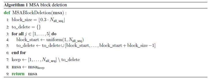
MSA block deletion
MSA의 row를 block 단위로 제거하여, 효과적으로 clade 단위의 정보를 제거한다. Data augmentation 관점에서 생각해볼 수 있다.
MSA의 row 각각은 한 species의 sequence를 나타낸다. 이 때, 맨 위의 sequence는 query sequence로 고정되고, 그 아래부터는 tool의 output (보통은 e-value)으로 정렬된다. 따라서 MSA에서 연속된 row들이 이루는 block을 없애는 것은, phylogeny 상에서 특정 branch 이하의 species를 통째로 없앨 가능성이 높다. Input의 diversity를 증가시키기 위해서, AlphaFold2에서는 매 input마다 random한 MSA row block을 제거한다.
MSA clustering
MSA row 개수를 줄이기 위하여 clustering한 뒤 대표 sequence를 활용한다.
Evoformer module이 필요로하는 memory cost는 이므로, 학습이 충분히 잘 되는 선에서 을 줄이는 것이 유리하다. Naive하게는 MSA의 row를 random sampling하면 되지만, 이러면 random subset에 선택되지 않은 sequence 때문에 information loss가 너무 크다.
Information loss를 최소화하면서 MSA의 row를 줄이는 방법은 없을까? 유사한 sequence들끼리 clustering하고, 각 cluster의 대표 sequence를 가져가는 전략을 취하면 된다.
자세한 방법은 여기를 참고
Residue cropping
MSA column(residue)의 일부 segment만 취해서 학습에 활용한다.
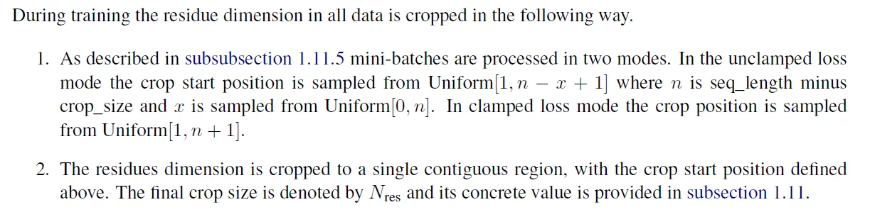
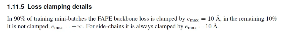
참고) Loss clamping
Input features
MSA feature와 pair feature는 다음과 같이 구성된다. 하나하나의 의미를 파악해보는 것도 좋을 것이다.
보기
Self-distillation dataset
PDB에 구조가 알려진 단백질들로 학습된 undistilled model을 이용하여, unlabelled data에 pseudolabel(or pseudo-structure?)를 붙이고 이를 학습에 활용한다.
Knowledge distillation의 motivation은 모델의 성능을 높이기 위해서, 많은 수의 model을 ensemble하거나 모델의 크기를 키우는 방법을 피하고자 함이다. 많은 수의 model prediction의 average를 prediction으로 사용하기보다는, 한 model(student)이 다른 model(teacher)의 output을 모방하도록 training 시킴으로써, teacher model이 학습한 knowledge를 student가 배울 수 있도록 한다. Output을 모방하는 것과, knowledge를 distillation 시키는 것과 무슨 상관이 있을까?
좋은 설명을 해둔 블로그가 있다. 간단히 요약하자면, teacher output으로 나타난 soft-label 자체에, teacher가 학습한 feature(knowledge)에 대한 단서가 녹아 있다는 것이다. 예를 들어, 어떤 이미지에 대해서 teacher의 예측 결과가 '고양이' class에 대해 0.7, '강아지'에 대해 0.25, 그리고 '컵'에 대해 0.05 였고, 이러한 비슷한 경향성을 보이는 input image가 충분히 존재한다면, student network는 teacher의 output에 의해서 다음과 같은 knowledge를 배울 수 있을 것이다:
"고양이는 컵보다 강아지와 더 비슷하구만!"
이러한 관점에서 'Distillation'이라는 이름을 붙인 것은 절묘한 analogy인 듯 하다. Teacher의 output에는 knowledge가 녹아 있고, 이를 모방하고자 학습하는 과정에서 그 안에 녹아 있는 knowledge를 얻게 되는 것이다. 추가적으로, teacher output의 softmax를 취할 때 temperature parameter 를 조절해주어,
probability distribution이 knowledge가 distill될 수 있을만큼 충분히 soft하게 만들어주는 trick이 사용된다. 이 또한 재미있는 은유라고 볼 수 있겠다.
Teacher의 지식을 student에 전해준다는 점에서, knowledge distillation은 위의 설명으로 비교적 이해가 가능하다. 그렇다면 self-distillation (SD) 은 어떻게 이해하면 될까? 스스로의 output을 같은 모델이 예측하도록 만드는 것이 과연 어떤 의미가 있길래 (Teacher 모델이 student보다 크지 않은데도!), 이 방법론이 2019년 이후 주목받기 시작한 걸까?
openaccess.thecvf.com
https://openaccess.thecvf.com/content_ICCV_2019/papers/Zhang_Be_Your_Own_Teacher_Improve_the_Performance_of_Convolutional_Neural_ICCV_2019_paper.pdf
Be Your Own Teacher: Improve the Performance of Convolutional Neural Networks via Self Distillation (Zhang et al., ICCV 2019)
이 논문에서 제시하는 self-distillation 방법. Prediction output을 teacher로 삼고, shallow layer + prediction head의 output을 student로 삼아서 자신의 final output을 자신의 shallow output으로부터 예측 가능하게 학습시킨다.
위의 논문에서는 놀랍게도 KD보다 SD의 경우 더 빠르게 학습되고 성능도 더 좋다고 한다.
원인이 궁금한데, 논문의 discussion에서는 다음과 같이 제시하고 있다.
•
SD can help models converge to flat minima which features in generalization inherently
→ Weight에 gaussian noise를 주는 실험으로, SD로 학습된 모델의 성능이 weight의 noise에 더 robust하다, 즉 loss의 flat minima (not sharp)에 존재한다는 것을 보여줌.
•
Self distillation prevents models from vanishing gradient problem
•
More discriminating features are extracted with deeper classifiers in self distillation
이런 논의들이 의미가 있기는 하지만... Self distillation이 어떻게 이런 결과에 관여했는지, causual relationship을 보인 결과는 아니라 만족스럽지는 못하다. 왜 SD가 성능을 향상시키는 걸까?
이 논문은 AlphaFold2 paper에서 cite하고 있는 논문이다. Self-distillation 방법론을 이 논문과 유사하게 했다고 하는데,
간단히 요약하자면, student model이 학습하는 pseudolabeled data에 noise를 추가하면 teacher model의 크기와 같거나 큰 student model을 학습할 수 있으며, 성능도 teacher보다 더 잘 나온다는 것이다. (청출어람!)
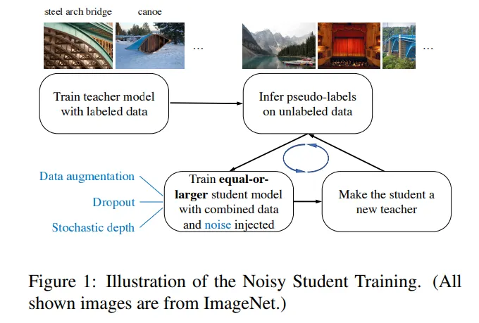
Noisy student training의 개요. 먼저 labeled data로 teacher model을 학습시키고, unlabeled data의 pseudo-label을 예측하게 한다. 그 다음, labeled + pseudolabeled 데이터셋을 이용하여 student model을 만드는데, 이 과정에서 data augmentation을 통해 noise를 추가한다. 이렇게 학습된 student를 새로운 teacher로 하여 model을 refine하는 과정을 반복한다.
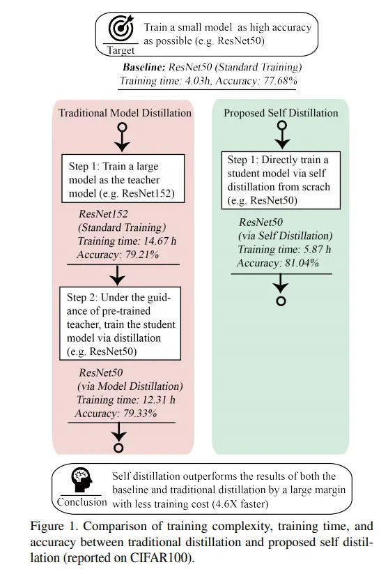
우선, 느낀 점은 AlphaFold2 논문의 self-distillation의 정의가 다소 모호하다는 것이다. ICCV 2019 논문의 경우 모델이 딱 하나로 정해져있고, training 도중 self-distillation loss와 output prediction loss가 동시에 작용하여 parameter를 update하는 반면, AlphaFold2에서 말하고 있는 self-distillation의 경우 undistilled model (구조가 알려진 PDB로 학습된)을 이용하여 구조가 알려지지 않은 input들의 pseudo-structure를 예측하는 방식이다. Undistilled model의 label(단백질의 구조)을 사용하는 거니까, 엄밀하게 self-distillation이라 말하기 모호하기는 한데... noisy student training framework에는 딱 들어맞는 방법론이긴 하다.
아래는 논문 experiment 주요 결과이다.
•
Noise injection (data augmentation)의 중요성
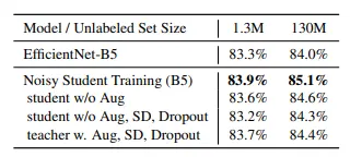
Student가 teacher보다 성능이 잘 나오려면, 충분한 noise가 필요하다는 것을 보여준다.
•
Iterative training의 중요성
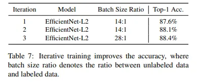
Noisy student를 새로운 teacher로 삼아 training하는 iteration이 1→2→3 순으로 많을 수록 성능이 좋아진다는 것을 보여준다.
•
Ablation study의 요약. (몇몇 당연한 사실들...?)
1.
Teacher model이 클수록 noisy student training의 성능이 좋다.
2.
Unlabeled data가 많아야 성능이 좋다.
3.
Soft pseudolabel이 몇몇 out-of-domain data case들에서 더 잘 작동한다.
4.
Size가 큰 student model은 powerful model을 학습하는 데 중요하다.
5.
Small model의 경우 data balancing이 중요하다.
6.
Labeled data와 unlabeled data를 함께 dataset에 두고 joint-training하는 것이 unlabeled data로 먼저 training하고 labeled data로 fine-tuning하는 것보다 좋다.
→ 이건 쓸모있는 결과인듯!
7.
Unlabeled : labeled batch size의 비율이 클수록 unlabeled data에 대해서 더 많이 학습되게 하고, 성능이 더 좋아진다.
8.
Student를 teacher weight로 initialize하는 것보다, scratch부터 training하는 것이 종종 더 좋다.
→ 이것도 눈여겨봐두자.
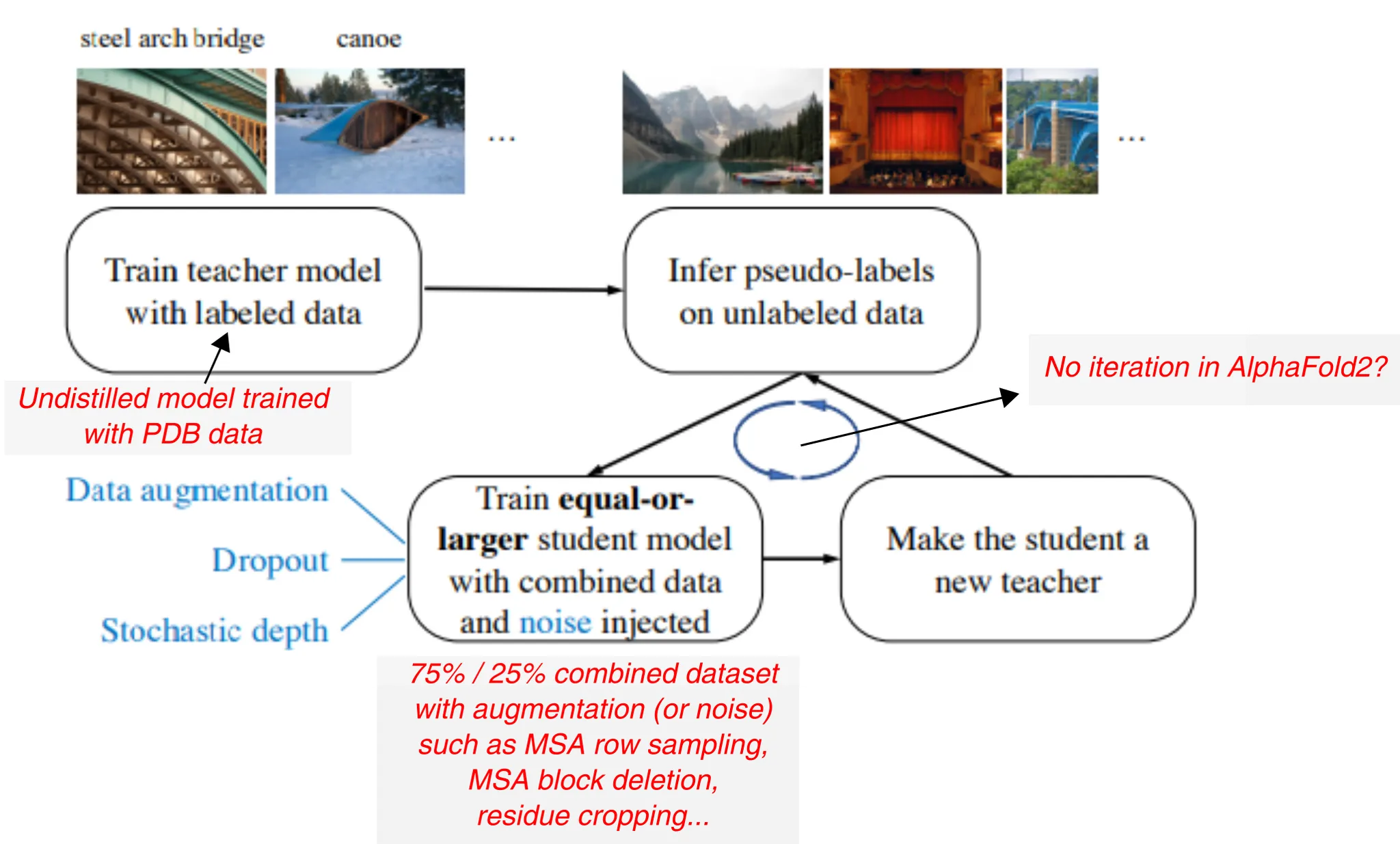
이 그림은 AlphaFold2의 맥락에서 noisy student training이 어떻게 이루어지고 있는지 보여준다. 단, AlphaFold2는 unlabeled data의 training에의 활용에만 방점을 찍고 있는 것인지, 학습된 student model로 다시 pseudolabel 만들고 training 하는 iteration은 사용하지 않는 것으로 보인다.
Evoformer stack in detail
MSA row-wise gated self-attention with pair bias
MSA representation의 row 단위로 gated self-attention을 수행하는데, pair representation의 linear projection을 bias로 반영하여 attention weight를 구하게 된다.
Pair에 관한 prior knowledge를 self-attention에 반영시키는 이 방법을 잘 기억해두자.
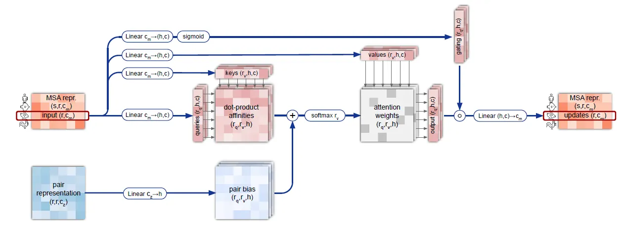
MSA row-wise gated self-attention with pair bias 연산의 흐름도.
Pseudocode
MSA column-wise gated self attention
단순히 MSA representation의 column 단위로 gated self-attention을 수행한다.
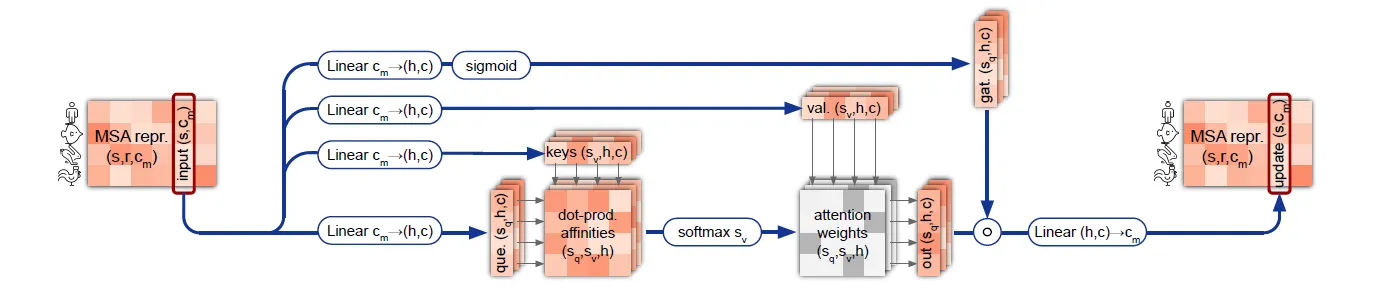
MSA column-wise gated self attention 연산의 흐름도.
Pseudocode
Outer product mean 연산이란?
MSA representation 상의 column pair의 relationship 정보를 pair representation에 전달한다.
참고) 반대로 pair representation의 정보를 MSA로 전달하는 건 MSA row-wise gated self attention에서 수행된다. 즉 서로의 정보가 하나의 iteration 상에서 왔다갔다 이동하는 것이다.
Outer product mean의 context는 아래 그림과 같다. 즉, axial self-attention + transition을 거친 MSA representation을 pair representation에 더해주기 위해서, pair representation 과 같은 dimension r x r 로 변환하는 것이 1차적인 목적이라고 할 수 있겠다.
다만, MSA representation의 all-pairwise column pair에 대한 outer product → mean 연산을 통해 해당 column pair의 relationship에 대한 information을 차원으로 embedding하는 것이 핵심이다.
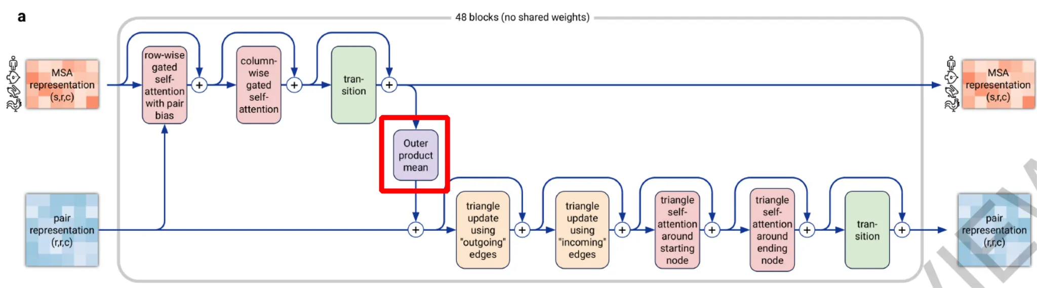
Outer product mean 연산의 context. 위 그림은 Evoformer block 구조를 나타내며, outer product mean 연산을 붉은 네모로 표시해두었다. MSA representation 정보를 pair representation에 더해주기 위해 필요한 연산임을 알 수 있다.
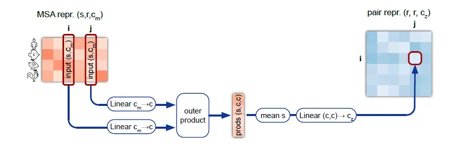
Outer product mean 연산의 흐름도.
왜 outer product를 썼을까? 두 vector representation의 outer product에 어떤 의미가 있어서 이 연산에 outer product를 써야겠다고 생각했던 걸까?
사실 이 연산은 AlphaFold2에서 처음으로 사용된 것이 아니라, 'rawMSA: End-to-end Deep Learning using raw Multiple Sequence Alignments' 이라는 논문에서 처음으로 사용된 것으로 보이며,(https://journals.plos.org/plosone/article?id=10.1371/journal.pone.0220182), CopulaNet (https://www.nature.com/articles/s41467-021-22869-8) 등의 모델에서도 나타난다.
아래 논의는 CopulaNet 논문을 참조하였다.
Outer product mean 연산에서 우리가 알고 싶은 것은, 두 column의 embedding들이 co-vary하는가이다. MSA representation feature는 주로 mutation이 있냐/없냐 정보를 가지기 때문에, 이 말인즉슨 두 residue가 co-evolve하는가를 나타내게 된다. 다시 말해, 한 쪽 residue에 mutation이 있을 때, 다른 쪽 residue에도 mutation이 같이 존재하는지를 알고싶은 것이다. 이 경우, representation vector 간의 all-pairwise 곱을 구하게 되면, mutation이 동시에 존재하는 경우에는 값이 클 것이고, 한쪽이라도 mutation이 없는 경우에는 값이 작아질 것이다. 따라서 outer product는 두 column의 co-evolution을 측정하는 데 매우 적절한 연산이다. 실제로 CopulaNet에서는 이를 'Co-evolution aggregator'라고 이름붙였다.
Pseudocode
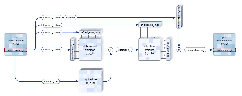
Triangular multiplicative update란?
Edge 하나를 self-attention-like하게 update할 때, 해당 edge와 함께 삼각형을 이루는 다른 두 edge들을 동시에 고려하면서 update하는 방법.
기본적으로 이 연산은 self-attention 관점에서 이해하면 될 듯 하다. Pair representation을 update하는 연산이므로, residue-pair를 나타내는 edge에 대한 self-attention으로 보자.
Naive하게 다른 모든 edge를 보고 (flattening → self attention) update하거나, axial attention으로 update하면 되지 않나? 생각할 수 있다. 실제로 가능하지만, 이렇게 하면 성능이 떨어진다는 것이 ablation study결과로 나와 있다. (Fig. 4a)
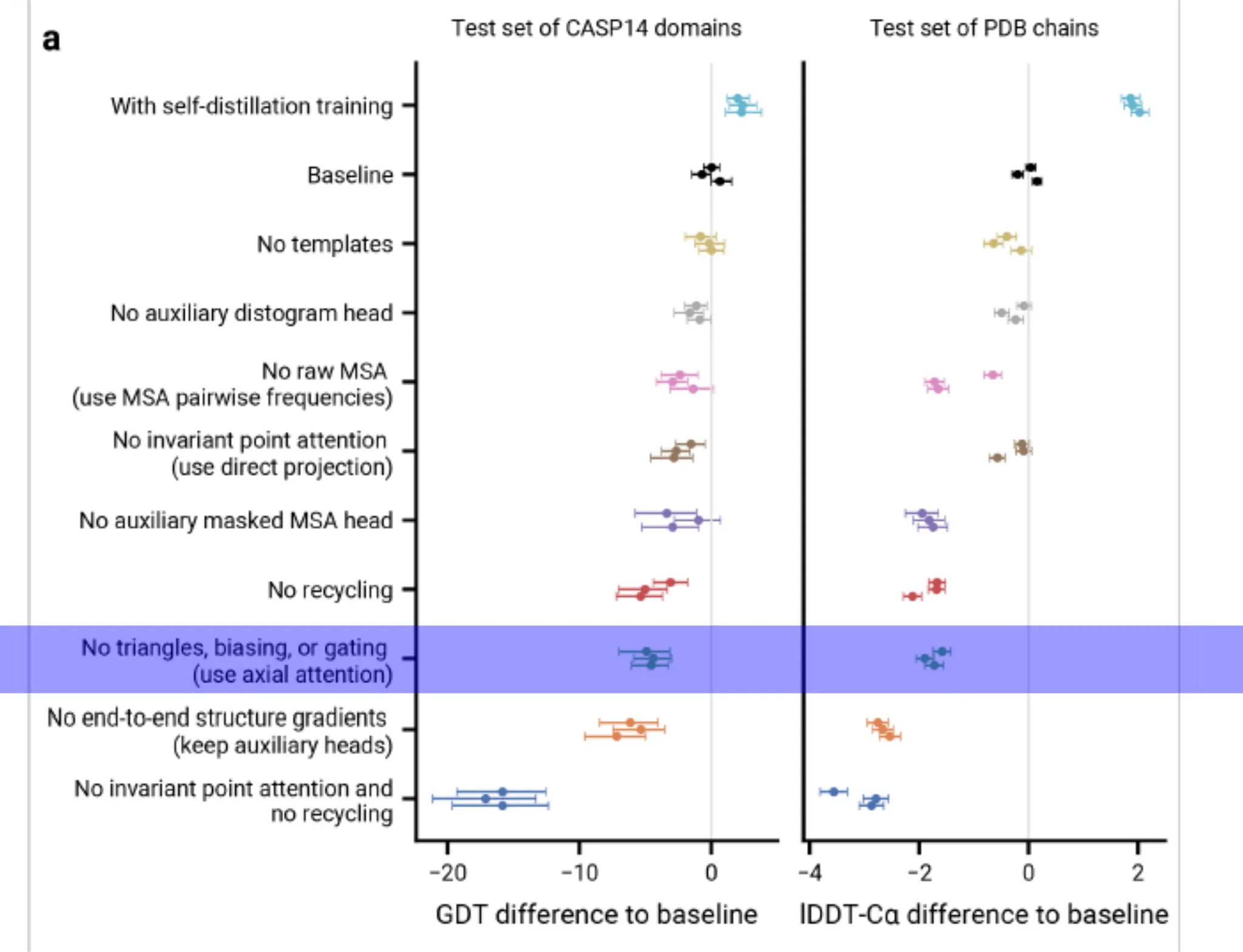
Fig. 4a. Ablation study 결과
그럼 대체 triangular multiplicative update는 어떤 연산이고, 어떤 역할을 하길래 성능 향상에 많은 도움이 되는 것인지 알아보자.
Amino acid residue들이 만족해야 할 constraint들은 residue pair 단위에서 나타나기도 하지만, residue의 triplet 단위에서 나타나는 경우도 존재한다. 이를테면 residue 간 거리는 삼각부등식을 만족해야 한다. 이 조건은 pairwise attention으로는 모델 상에 반영될 수 없고, 하나의 edge를 update할 때 그 edge와 삼각형을 이루는 다른 두 edge를 동시에 확인할 때, 그제서야 해당 edge가 가지는 constraint를 확인할 수 있다. 따라서 저자들은 나머지 두 edge의 gated linear projection 값을 이용하여 edge를 update함으로써 이러한 정보가 pair representation 상에 효과적으로 반영될 수 있으리라 기대하였다.
이 때 edge ij가 포함된 삼각형의 edge들은 node i, j에서 나가는 edge들을 포함할 수 있고(outgoing), i, j로 들어오는 edge들을 포함할 수 있다(incoming). 이 symmetry를 반영하기 위해서 triangular multiplicative update는 outgoing edge에 대해서 한 번, incoming edge에 대해서 한 번, 총 두 번 수행하게 된다.
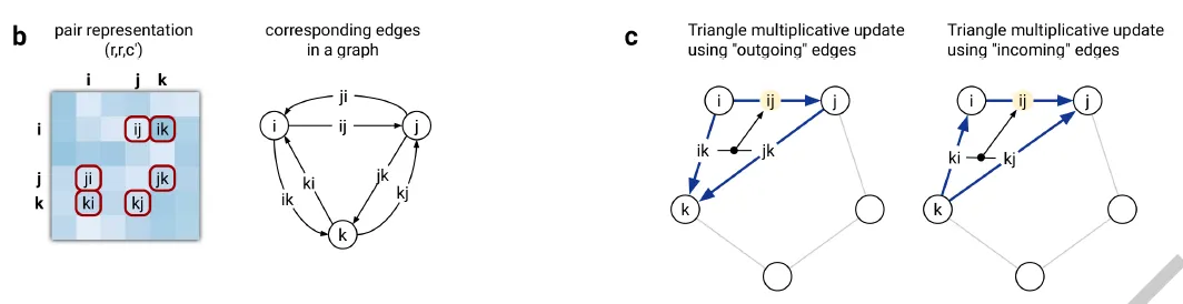
Triangular multiplicative update의 모식도.
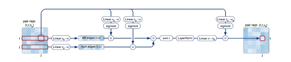
Triangular multiplicative update using "outgoing" edges. Edge ij 와 삼각형을 이루는 edge들, ik와 jk에 대해서 linear projection을 gating한 후 inner product를 구하고, 한번 더 gating한 이후 값들을 aggregate함으로써 이루어진다.
Pseudocode
Triangular self-attention이란?
Starting/Ending node 하나를 공유하는 두 edge의 affinity를 query-key dot product로 계산하고, 삼각형을 완성하는 나머지 edge의 정보를 bias로 추가하여 해당 starting/ending node를 중심으로 하는 삼각형의 attention을 계산한다.
Triangular self attention의 경우도 triangular multiplicative update와 마찬가지로, 삼각형을 이루는 edge 관계를 함께 보고자 함이 목적이다. 이 경우는 self-attention framework 상에 두 종류 edge 정보를 동시에 반영시키는 것이 특징이다. 어떻게 이를 구현했는지 보자.
Triangular self-attention에서는 기준을 edge 를 구성하는 두 node 와 로 한다. 즉, node 를 공유하는 다른 모든 edge들 와 (around starting node), node 를 공유하는 다른 모든 edge들 를 고려하여 (around ending node), 두 번의 symmetric한 self-attention 연산을 연속적으로 수행하게 된다.
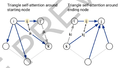
Triangular self-attention의 모식도.
한 edge를 update할 때 starting node를 공유하는 edge 하나하나씩을 보려면, pair representation의 row 하나에 대해서 단순히 query-key-value를 쓰는 standard self-attention을 써도 충분하다. 이를 확장하여 두 edge를 동시에 보고 attention을 수행하려면, 어떻게 해야 할까?
간단하다! 이 추가적인 edge (아래 그림에서 right edges로 표현된)에 대한 (linear projection된) 정보를 dot-product affinity에 bias term으로 추가해주면 된다.
이런 형태로. edge ij가 query, ik가 key인 scaled dot product에 jk가 나타내는 bias term이 추가된 것을 확인하자.
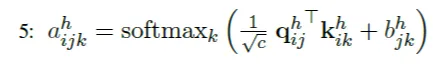
정리하자면 아래 그림의 dot-product affinities의 element 는 Edge 와 의 affinity를 나타내며, bias term의 element 는 edge 가 주는 bias를 나타낸다. 따라서 이 두 matrix를 더하게 되면 자연스럽게 attention weights 는 가 이루는 삼각형의 attention을 나타내게 되는 것이다.
Triangular self-attention around starting node. Edge ij의 representation을 update할 때, starting node i를 공유하는 다른 모든 edge ik들에 대한 query-key affinity를 이용한다. 더불어서,
Pseudocode
Structure Module in detail
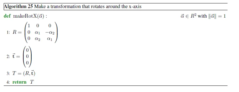
Construction of frames from ground truth atom positions
Ground-truth position을 생성하기 위하여 atom coordinate으로부터 backbone frame들을 계산한다.
Gram-Schmidt process를 이용하여 ground truth atom position으로부터 residue를 나타내는 backbone frame을 계산하는 방법이다. 해당 backbone frame 좌표계의 원점은 항상 이다.
Pseudocode
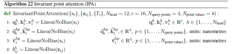
Invariant point attention (IPA)
두 residue 사이의 attention을 3차원 공간에서 수행하되 3차원 공간 자체의 global transformation에는 invariant하고, 두 residue의 상대적인 거리가 변화할 때에만 attention이 변화할 수 있도록 하는 것이 목적이다.
두 개의 residues 를 생각하자. 이 모듈의 목적은 두 residue 사이의 information을 어떻게든 반영한 self-attention을 통하여 single MSA representation을 update하는 것이다.
그러면 지금까지 만들어낸 feature들로부터 residue 사이의 관계를 어떻게 얻어낼 수 있을지 생각해보자.
1.
(Standard self-attention) Single MSA representation을 이용하여 standard self-attention (query-key-value)을 수행하여 udpate할 수 있을 것이다. (아래 그림, red highlight)
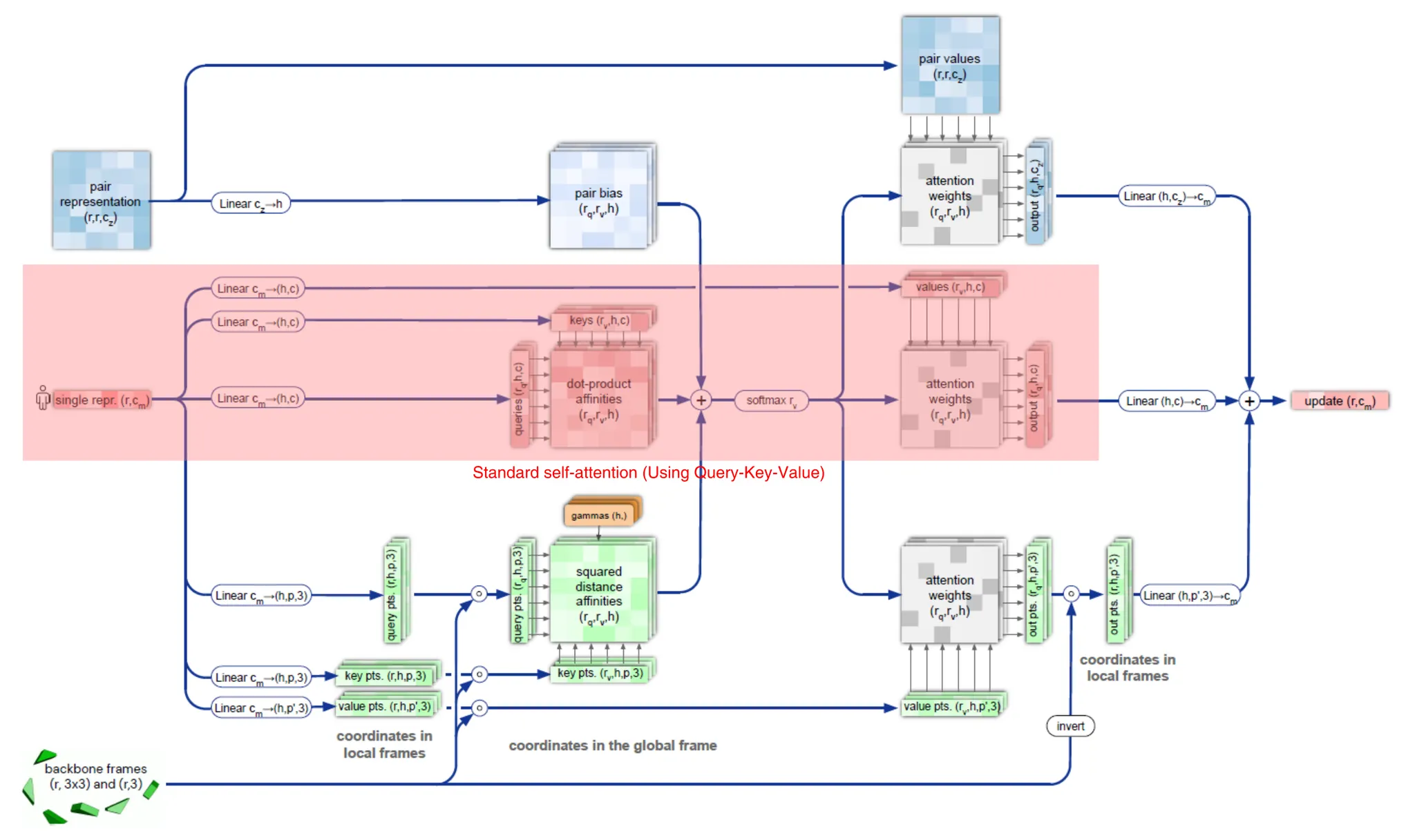
Standard self-attention of single MSA representation.
2.
(Modulation by pair representation) Pair representation을 scaled dot-product로 생각하여, Softmax 직전에 bias term으로 추가해줄 수 있다. (아래 그림, blue highlight)
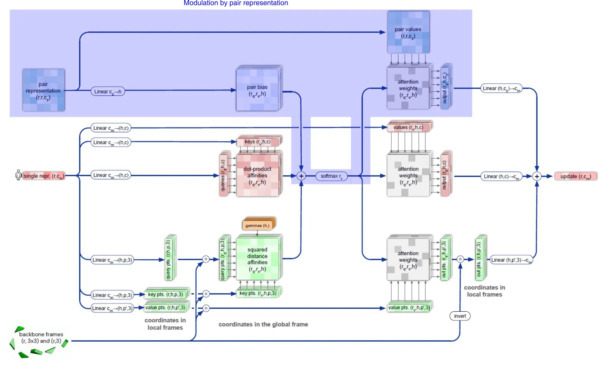
Modulation by pair representation.
3.
(Invariant point attention; IPA) Residue 의, 현재까지 예측된 3차원 상의 backbone frame 사이의 관계 (거리가 가까울수록, 보다 많은 관계성을 부여)를 self-attention 상에 반영할 수도 있다. (아래 그림, green highlight)
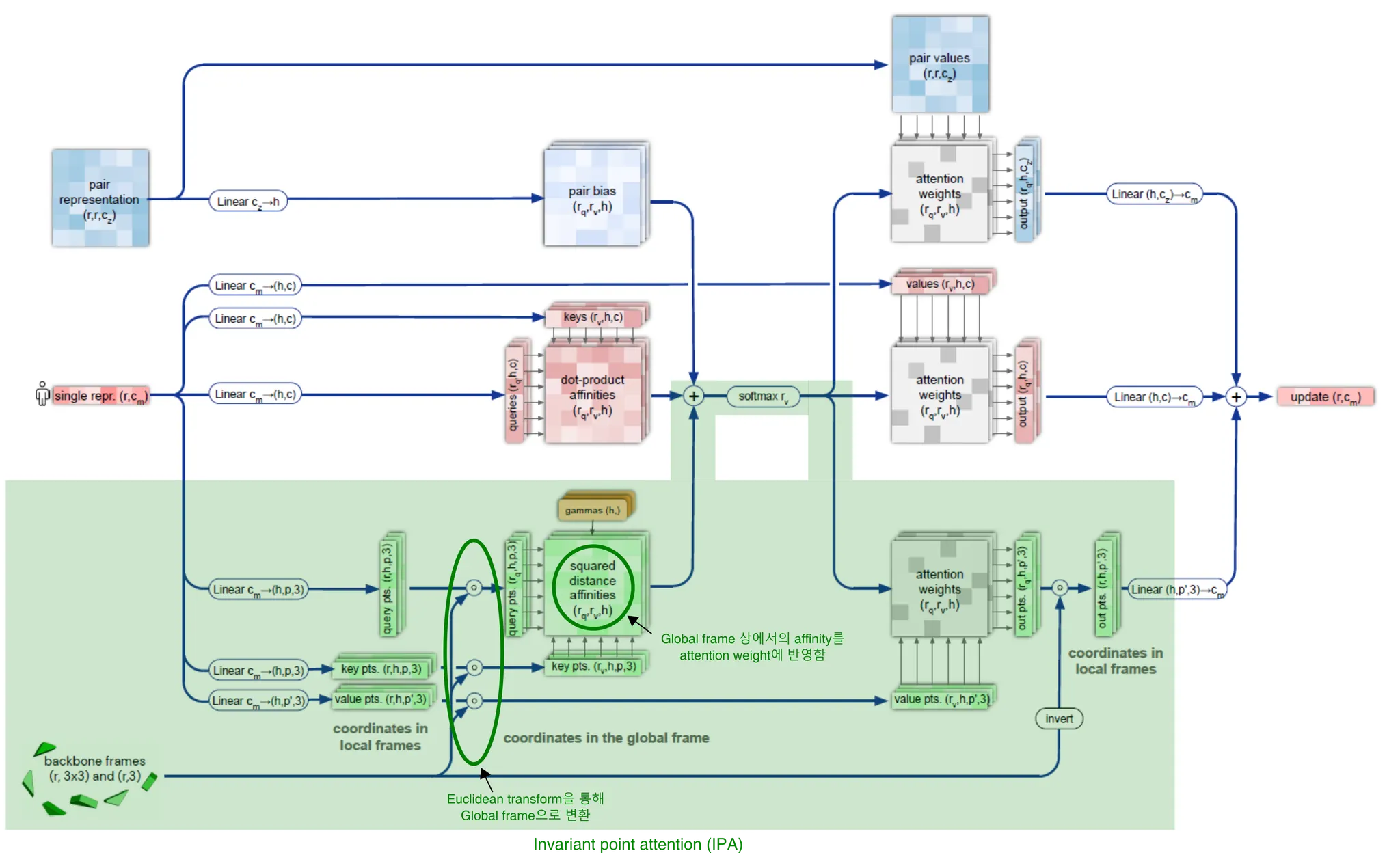
Invariant point attention.
IPA는, 간단히 말해 attention을 3차원 공간에서 수행하되 3차원 공간 자체의 global transformation에는 invariant하고, 두 residue의 상대적인 거리가 변화할 때에만 attention이 변화할 수 있도록 하는 것이 목적이다.
보다 구체적으로 설명하자면 아래와 같다. Single MSA representation의 column 를 적절히 linear projection시켜서 (LinearNoBias 연산 이용), backbone frame 상에서 적절하게 임의의 point 를 sampling할 수 있다고 생각해 보자. 다음 pseudocode의 2, 3번째 줄처럼 말이다. 이것의 의미는, amino acid residue의 위치 근처의 point를 3차원 공간 상에서 sampling한 것으로 생각하면 된다. (단, point를 나타내는 3차원 좌표계는 각 residue의 backbone frame을 이용한다.)
보통의 self-attention의 경우 input feature를 linear projection한 query와 key의 affinity를 (scaled) dot-product로 구한다. 하지만 IPA의 경우 해석이 오히려 straightforward하다.
두 residue가 가깝다면, sampling된 point 또한 가까울 것이고, 따라서 global frame 상에서 두 point의 거리는 가까울 것이다. 따라서 두 residue 에 높은 attention weight을 준다.
여기서 한가지, 와 는 각각 local backbone frame 상에서 sampling된 것이기 때문에, 이를 global frame 상에서의 coordinate으로 변환해주기 위해서는 각 local backbone frame의 transformation을 이용하여 변환해주어야 한다.
→ 형태는 따라서 global frame에서의 point 의 coordinate을 나타낸다.
결과적으로 두 residue 사이의 squared distance affinity는 아래 식으로 계산되며, 이 값을 적당히 normalize하여 self-attention의 bias로 사용한다.
증명) 이 term은 global transformation-invariant하다.
직관적으로 생각해봐도, 두 점 사이의 거리는 두 점에 동일한 rigid transform (회전변환, 평행이동)이 주어진다는 전제 하에 global transformation-invariant하다.
식으로 보자면, 각 point에 global transformation을 적용시키면 아래 식과 같다.
여기서, vector의 L2-norm은 rigid transformation에 invariant하기 때문에 다음이 성립한다. (결국 말로 풀어서 한 것과 같은 소리다...)
위의 세 가지 의 관계를 다음과 같은 형태로 self-attention에 반영하면 된다! Full pseudocode는 아래 참조.
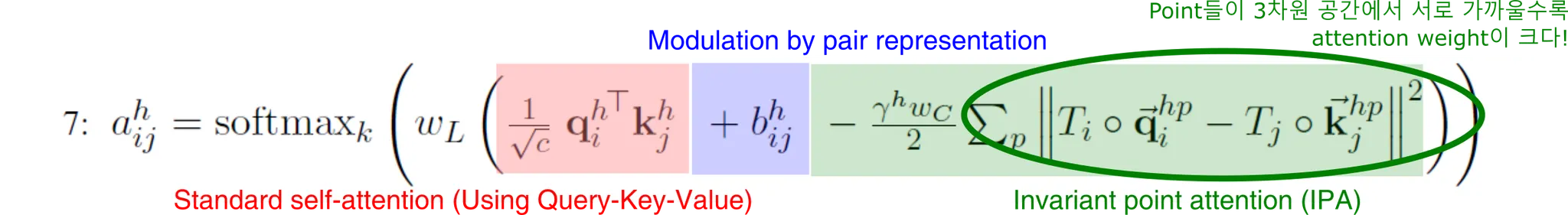
AlphaFold2에서 어떻게 MSA, residue pair information이 3D structure로 반영될 수 있는지를 나타내는 핵심 식이다. 아마도 AlphaFold2 구조 상에서 가장 중요한 식이 아닐까 싶다. 모든 information이 self-attention의 inductive bias term의 형태로 하나로 집약되므로!
Pseudocode
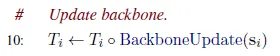
Backbone update
MSA single representation으로부터 update transformation을 예측하고, 이를 활용하여 backbone frame을 update한다.
Backbone frame을 update하는 transform을 예측하는데, 방법은 매우 간단하다.
Update된 MSA single representation의 column 를 linear projection하여 사원수(Quarternion)를 예측하고 이를 이용해 rotation matrix 을 만든다. Translation vector 는 그냥 예측한다.
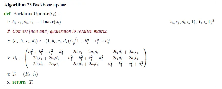
Update transform을 구했으면 다음과 같이 적용시킨다.
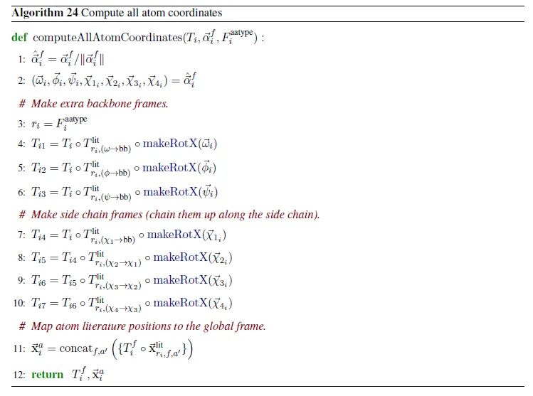
Atom coordinate computation
MSA single representation으로부터 각 amino acid residue별 torsion angle을 예측하고, 이로부터 atom의 coordinate을 계산한다.
제일 먼저, 와 의 nonlinear combination을 이용해서 torsion angle들을 예측한다.
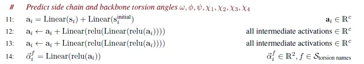
그리고 아래 식을 이용하여 atom의 위치를 결정하면 끝이다.
이후의 후처리 작업들은 다소 minor한 내용이라 여기서는 다루지 않겠다.
Loss functions and auxiliary heads
Network는 end-to-end로 training되므로, 각 weight의 gradient가 계산되어 올 loss를 잘 정의하는 것이 중요하다. 핵심 loss는 structure 예측을 얼마나 잘 했는지에 대한 frame aligned point error (FAPE) loss이지만, 많은 수의 auxiliary loss들이 존재하여 intermediate weight의 training이 안정적으로 이루어질 수 있도록 돕는다.
Training 시와 fine-tuning 시의 loss는 아래와 같이 약간 다르다.
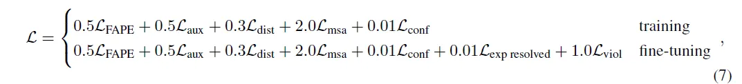
Loss term이 이렇게 많은 이유는 무엇일까?
저자들이 언급하기로는, FAPE, aux, distogram, MSA loss의 경우에는 모델의 major subcomponent 각각에 대해서 해당 모듈이 만들어진 목적 그대로 학습이 잘 이루어질 수 있도록 individual loss를 추가해준 것이라고 한다. 이 loss들이 정말 다 필요할까? Ablation 해봤나?
→ Ablation result (Figure 4a of the main text)
각 loss term의 의미와 목적하는 바를 설명하면 다음과 같다.
•
: Frame aligned point error
→ Local frame 상에서의 원자의 상대적인 위치를 ground truth와 비교하여 loss로 계산한다.
•
: Auxiliary loss from the Structure Module
→ Averaged FAPE and torsion losses on the intermediate structures
•
: Averaged cross-entropy loss for distogram prediction
→ Residue pair representation이 진짜로 residue 와 의 관계를 학습한다는 것을 보장하여, Structure module에서 confident하게 잘 사용될 수 있도록 한다.
•
: Averaged cross-entropy loss for masked MSA prediction
→ BERT-loss
→ Inter-sequence or phylogenetic relationship을 모델이 학습하도록 한다. 즉, co-evolution을 잘 학습하도록 한다.
→ 다른 covariance statistic을 안 넣어주고도 모델을 원하는 방향으로 guide하는 elegant한 방법이라고 생각된다.
•
: Model confidence loss
→ 이 loss 덕분에 per-residue accuracy of the structure (pLDDT)를 만들 수 있었다.
•
: "Experimentally resolved" loss
→ ?? 잘 모르겠다
•
: Violation loss
→ 모델이 physically plausible structure를 만들도록 한다.
구현 상의 detail을 설명하면 아래와 같다.
•
길이가 짧은 sequence들의 중요도를 낮추기 위해서, 각 training sequence의 final loss에 해당 sequence의 길이의 제곱근을 곱해준다.
•
Weight는 hand-selected 되었고, 거의 변화시키지 않았다.
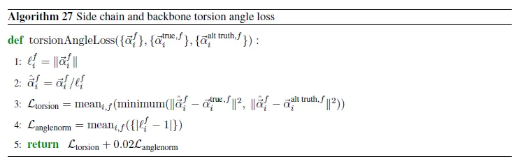
Side chain and backbone torsion angle loss
Atom의 torsion angle이 truth와 얼마나 비슷한지 측정하는 loss. 몇 가지 trick들이 적용되었지만 여기서는 다루지 않겠다.
Frame aligned point error (FAPE)
예측된 local frame 하에서 예측된 atom coordinates 와 ground truth frame 하의 atom coordinates 이 얼마나 가까운지 계산하는 loss
즉, local frame이 주어졌을 때 atom의 상대적인 위치들을 비교하는 loss이다.
먼저 알고리즘을 보자.
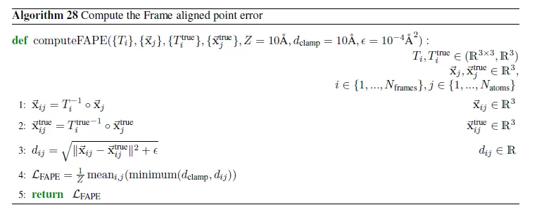
1번 줄은 atom 의 global coordinate 를 local frame 하에서의 local coordinate 으로 변환하는 과정이다. 2번 줄도 마찬가지로 ground truth에 대해서 같은 연산을 수행하는 것이다.
3번 줄에서는 L2-norm으로 두 local coordinate 사이의 거리를 측정하여, 최종 loss는 4번 줄에서 clamped L1-loss의 형태로 구해지게 된다.
이 loss 또한 global rigid transformation-invariant하다는 사실은 자명하다. 근데 reflection에도 invariant할까?
invariant하지 않다 → 설명
→ 따라서 AlphaFold2가 chirality도 고려하게 된다.
Model confidence prediction (pLDDT)
FAPE loss를 에 대해서만 수행하는 cheap version의 FAPE loss를 lDDT-라 한다. AlphaFold2는 residue 단위로 lDDT-가 얼마나 될지 예측하는 intrinsic model accuracy estimate이 존재하는데, 이를 pLDDT라 부른다.
Additional head를 달아서 per-residue lDDT-값을 binning하여 classification 문제로 바꾼 뒤 예측하게 하며, cross entropy loss 로 학습이 이루어진다.
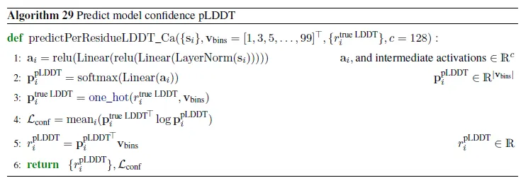
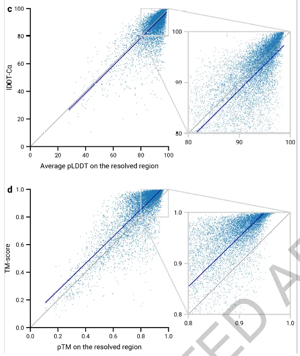
Fig 2c,d. (c) pLDDT와 lDDT-Ca가 잘 비례함을 알 수 있다. (d) 아래는 pTM 예측 또한 가능함을 보여주고 있다. 여기서는 다루지 않음.
Distogram prediction
Pair representation ()에 대해 계산된다. 먼저 pair representation을 symmetrize하고 (), matrix를 linearly project하여 64개의 distance bin (2Å~(>22Å)을 64등분)에 속할 probability를 계산하도록 한다. Target은 정답 distance가 속하는 bin을 나타내는 one-hot vector이고, loss는 all residue pair 에 대한 distance prediction의 cross entropy.
Masked MSA prediction (BERT-loss!)
Final MSA representation을 이용해서 masking된 (input embedding section 참조) amino acid를 예측한다. Target은 총 23개 (20개 amino acid + unknown + gap token + mask token). MSA representation을 output class로 linear projection하여 softmax를 취하고, cross-entropy loss를 구한다.
"Experimentally resolved" prediction
Atom의 위치가 high-resolution structure 내에서 experimentally resolve되었는지 예측하는 loss. Evoformer stack의 결과로 나온 MSA single representation 를 input으로 하여 atom-wise probability를 예측한다. Target은 High-resolution X-ray crystal과 cryo-EM structure (resolution <3Å) 결과로 residue 내의 atom이 resolved된 경우 1, 아닌 경우 0.
왜 필요할까??

Structural violations
Atom clash를 막기 위한 추가적인 loss. 자세한 내용은 아래 참조.
자세한 설명
Recycling in detail
Recycling은 본질적으로 network를 unfold하여 (RNN에서 하듯이) execution을 여러 번 수행하는 것이다. 다만, residual connection처럼 raw input feature는 매 fold마다 지속적으로 공급되고, parameter update에 사용되는 gradient 계산은 오직 마지막 recycling iteration에서 계산된 gradient만 사용된다는 점이 다르다.
대충 그려서 조잡해보이긴 하지만..Recycling을 위해 Evoformer와 Structure module을 1회 unfold한 모델은 아래 그림과 같다.
Recycling을 위해 1회 unfolded된 AlphaFold2 모델 구조.
Training과 inference 시의 recycling procedure의 pseudocode는 다음과 같다.
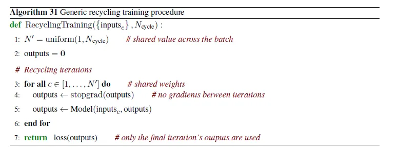
Training 시의 recycling 방법. 마지막 iteration의 gradient만 살아남는다는 것과, Line 1에 의해 같은 input이라도 recycling cycle 수가 random하게 매 batch마다 달라진다는 점에 주목하자.
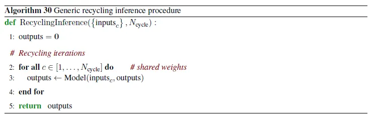
Inference 시의 recycling 방법.
Results
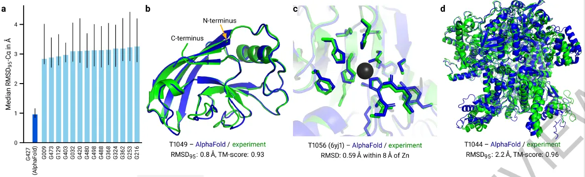
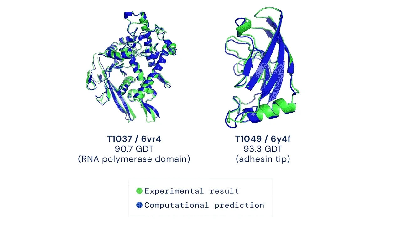
Fig 1a-d. (a) 성능이 좋다. (b-d) 예측을 잘한다.
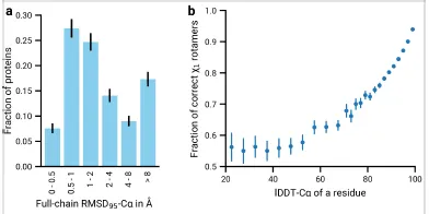
Fig 2a,b. (a) Overall median RMSD = 1.86Å. (b) Residue 위치 예측이 정확할수록 (backbone frame) atom torsion angle 예측이 정확해짐을 알 수 있다.
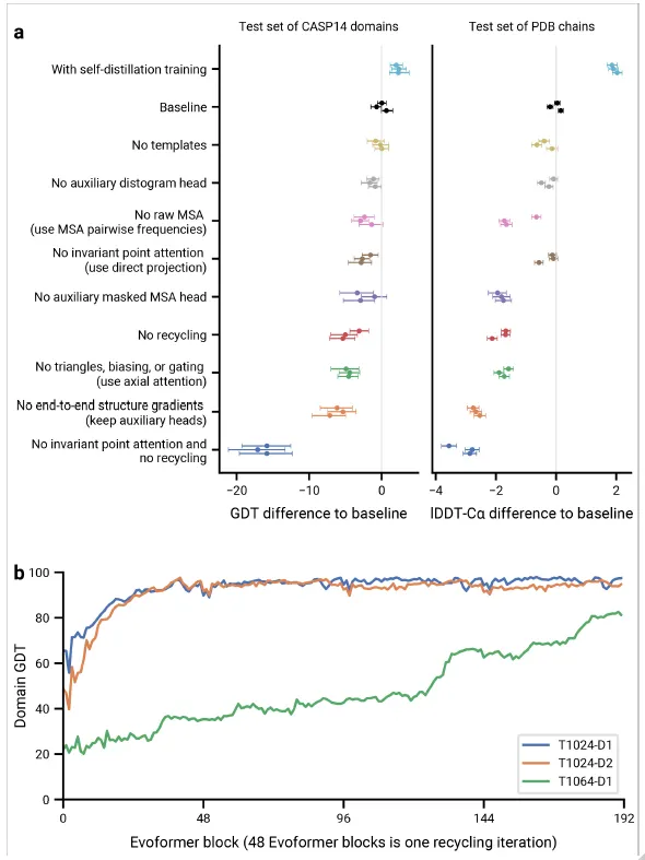
Fig 4a,b. (a) Ablation experiment. (b) Recycling의 필요성. 1cycle = 48 blocks.
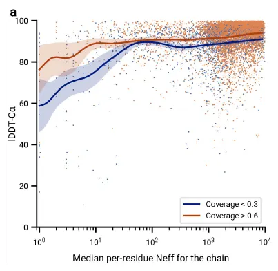
Fig 5a. MSA의 중요성. x축 → Effective한 MSA상의 sequence 개수. y축 → lDDT-Ca (backbone 예측에 대한 척도). Coverage = template coverage를 의미